Generating Channel Graphs for KlustaKwik Automatically
03 July 2015
In order to build the masks for KlustaKwik, SpikeDetekt2 needs to know the graph of adjacencies between all of the recording sites on a recording array. However, a bad channel for a recording session can drastically change the requirements for a probe geometry.
Luckily, there’s some math out there that can help us to build these adjacency matrices based solely on the geometry of the recording sites. I’ve already demonstrated how to use Delauney triangulation to do this for electrode arrays that are very large, where it would be a burden to define the geometry by hand. That was fun, but the technique has an application that I’ve already implemented into my own pipeline to extract population spiking activity.
We start with site maps in terms of Neuronexus recording sites
We are using we NeuroNexus probes. The recording sites are 1-indexed, whereas KlustaKwik uses 0-indexed channels (where each channel is a column in a 2D array). Further, due to our hardware configuration, NeuroNexus “Site 1” doesn’t necessarily correspond to KlustaKwik’s “Channel 0”. So we are going to define a site map that gives us the channel/index for each neuronexus site. The dictionary s is composed of site:channel pairs, where ‘site’ is the Neuronexus recording site and ‘channel’ is the index of that site’s recording in the Klustakwik *.raw.kwd file.
# site:channel
s = {11: 0,
     12: 1,
     22: 2,
     10: 3,
     21: 4,
     23: 5,
     9: 6,
     13: 7,
     24: 8,
     8: 9,
     20: 10,
     25: 11,
     7: 12,
     14: 13,
     26: 14,
     6: 15,
     19: 16,
     27: 17,
     5: 18,
     15: 19,
     28: 20,
     4: 21,
     18: 22,
     29: 23,
     1: 24,
     16: 25,
     32: 26,
     2: 27,
     17: 28,
     31: 29,
     3: 30,
     30: 31,
     }
Sometimes you lose channels
Sometimes you don’t have all of your channels. Maybe a channel is bad on your headstage or you’re using one channel as a reference. Things happen. That shouldn’t prevent us from using the most complete adjacency matrix that we can.
We’re going pretend like we’ve have some dead (or unrecorded) sites by setting their channel to None
from numpy import random
from pprint import pprint

for dead_site in random.choice(s.values(),5):
    s[dead_site]=None

pprint(s)
{1: 24,
 2: 27,
 3: 30,
 4: 21,
 5: 18,
 6: 15,
 7: 12,
 8: 9,
 9: 6,
 10: 3,
 11: None,
 12: None,
 13: 7,
 14: 13,
 15: 19,
 16: 25,
 17: 28,
 18: 22,
 19: None,
 20: 10,
 21: None,
 22: 2,
 23: None,
 24: 8,
 25: 11,
 26: 14,
 27: 17,
 28: 20,
 29: 23,
 30: 31,
 31: 29,
 32: 26}
Define our probe geometry in terms of the site map
If I were to manually define the adjacencies for each site on the NeuroNexus A1x32-Poly3-6mm-50 probe, this is what I would sketch:
 (3)      (30)
  | \    / |
 (2)-(17)-(31)
  | /    \ |
 (1)-(16)-(32)
  | \    / |
 (4)-(18)-(29)
  | /    \ |
 (5)-(15)-(28)
  | \    / |
 (6)-(19)-(27)
  | /    \ |
 (7)-(14)-(26)
  | \    / |
 (8)-(20)-(25)
  | /    \ |
 (9)-(13)-(24)
  | \    / |
(10)-(21)-(23)
  | /    \ |
(11)-(12)-(22)
Each number is the NeuroNexus site number and I’ve drawn my edges between them. This particular probe is a grid, so I have each square drawn and (for the sake of completeness) each square is split into two triangles. For KlustaKwik, I would need to write these out as a list of tuples.
Instead, we’re just going to define the probe geometry, giving the x,y coordinates of each site, where s[1] indicates site 1. If a different electrophysiology rig has a different hardware configuration, this will change, so it’s more robust to define this geometry in terms of the NeuroNexus sites.
Even though KlustaKwik doesn’t care about the geometry dict (except to plot the channels in Klustaviewa), we do. We are going to generate the graph on the fly from this geometry information, so I’ve defined it in microns, where the lower left recording site (Site 11) is (0,0).
channel_groups = {
    # Shank index.
    0: {
        # List of channels to keep for spike detection.
        'channels': s.values(),

        # 2D positions of the channels
        # channel: (x,y)
        'geometry': {
            s[3]: (0,500), # column 0
            s[2]: (0,450),
            s[1]: (0,400),
            s[4]: (0,350),
            s[5]: (0,300),
            s[6]: (0,250),
            s[7]: (0,200),
            s[8]: (0,150),
            s[9]: (0,100),
            s[10]: (0,50),
            s[11]: (0,0),
            s[17]: (50,450), # column 1
            s[16]: (50,400),
            s[18]: (50,350),
            s[15]: (50,300),
            s[19]: (50,250),
            s[14]: (50,200),
            s[20]: (50,150),
            s[13]: (50,100),
            s[21]: (50,50),
            s[12]: (50,0),
            s[30]: (100,500), # column 2
            s[31]: (100,450),
            s[32]: (100,400),
            s[29]: (100,350),
            s[28]: (100,300),
            s[27]: (100,250),
            s[26]: (100,200),
            s[25]: (100,150),
            s[23]: (100,100),
            s[24]: (100,50),
            s[22]: (100,0),
        }
    }
}
pprint(channel_groups)
{0: {'channels': [24,
                  27,
                  30,
                  21,
                  18,
                  15,
                  12,
                  9,
                  6,
                  3,
                  None,
                  None,
                  7,
                  13,
                  19,
                  25,
                  28,
                  22,
                  None,
                  10,
                  None,
                  2,
                  None,
                  8,
                  11,
                  14,
                  17,
                  20,
                  23,
                  31,
                  29,
                  26],
     'geometry': {None: (100, 100),
                  2: (100, 0),
                  3: (0, 50),
                  6: (0, 100),
                  7: (50, 100),
                  8: (100, 50),
                  9: (0, 150),
                  10: (50, 150),
                  11: (100, 150),
                  12: (0, 200),
                  13: (50, 200),
                  14: (100, 200),
                  15: (0, 250),
                  17: (100, 250),
                  18: (0, 300),
                  19: (50, 300),
                  20: (100, 300),
                  21: (0, 350),
                  22: (50, 350),
                  23: (100, 350),
                  24: (0, 400),
                  25: (50, 400),
                  26: (100, 400),
                  27: (0, 450),
                  28: (50, 450),
                  29: (100, 450),
                  30: (0, 500),
                  31: (100, 500)}}}
Clean up the dead channels
We have a lot of Nones in there, indicating dead channels. Let’s strip those out.
new_group = {}
for gr, group in channel_groups.iteritems():
    new_group[gr] = {
        'channels': [],
        'geometry': {}
    }
    new_group[gr]['channels'] = [ch for ch in group['channels'] if ch is not None]
    new_group[gr]['geometry'] = {ch:xy for (ch,xy) in group['geometry'].iteritems() if ch is not None}

channel_groups = new_group
pprint(channel_groups)
{0: {'channels': [24,
                  27,
                  30,
                  21,
                  18,
                  15,
                  12,
                  9,
                  6,
                  3,
                  7,
                  13,
                  19,
                  25,
                  28,
                  22,
                  10,
                  2,
                  8,
                  11,
                  14,
                  17,
                  20,
                  23,
                  31,
                  29,
                  26],
     'geometry': {2: (100, 0),
                  3: (0, 50),
                  6: (0, 100),
                  7: (50, 100),
                  8: (100, 50),
                  9: (0, 150),
                  10: (50, 150),
                  11: (100, 150),
                  12: (0, 200),
                  13: (50, 200),
                  14: (100, 200),
                  15: (0, 250),
                  17: (100, 250),
                  18: (0, 300),
                  19: (50, 300),
                  20: (100, 300),
                  21: (0, 350),
                  22: (50, 350),
                  23: (100, 350),
                  24: (0, 400),
                  25: (50, 400),
                  26: (100, 400),
                  27: (0, 450),
                  28: (50, 450),
                  29: (100, 450),
                  30: (0, 500),
                  31: (100, 500)}}}
Build the adjacency graph from the probe geometry
Next, we’ll use SciPy’s built-in Delaunay Triangulation to construct a graph from the probe geometry
from scipy import spatial
from scipy.spatial.qhull import QhullError
def get_graph_from_geometry(geometry):

    # let's transform the geometry into lists of channel names and coordinates
    chans,coords = zip(*[(ch,xy) for ch,xy in geometry.iteritems()])

    # we'll perform the triangulation and extract the
    try:
        tri = spatial.Delaunay(coords)
    except QhullError:
        # oh no! we probably have a linear geometry.
        chans,coords = list(chans),list(coords)
        x,y = zip(*coords)
        # let's add a dummy channel and try again
        coords.append((max(x)+1,max(y)+1))
        tri = spatial.Delaunay(coords)

    # then build the list of edges from the triangulation
    indices, indptr = tri.vertex_neighbor_vertices
    edges = []
    for k in range(indices.shape[0]-1):
        for j in indptr[indices[k]:indices[k+1]]:
            try:
                edges.append((chans[k],chans[j]))
            except IndexError:
                # let's ignore anything connected to the dummy channel
                pass
    return edges


def build_geometries(channel_groups):
    for gr, group in channel_groups.iteritems():
        group['graph'] = get_graph_from_geometry(group['geometry'])
    return channel_groups

channel_groups = build_geometries(channel_groups)
print(channel_groups[0]['graph'])
[(2, 8), (2, 3), (3, 2), (3, 8), (3, 7), (3, 6), (6, 7), (6, 3), (6, 10), (6, 9), (7, 8), (7, 11), (7, 3), (7, 6), (7, 10), (8, 2), (8, 3), (8, 7), (8, 11), (9, 6), (9, 10), (9, 12), (10, 7), (10, 11), (10, 6), (10, 9), (10, 14), (10, 13), (10, 12), (11, 7), (11, 8), (11, 10), (11, 14), (12, 13), (12, 15), (12, 10), (12, 9), (13, 14), (13, 17), (13, 12), (13, 15), (13, 19), (13, 10), (14, 13), (14, 17), (14, 10), (14, 11), (15, 12), (15, 13), (15, 19), (15, 18), (17, 13), (17, 14), (17, 20), (17, 19), (18, 19), (18, 15), (18, 22), (18, 21), (19, 18), (19, 15), (19, 20), (19, 17), (19, 13), (19, 22), (19, 23), (20, 19), (20, 17), (20, 23), (21, 18), (21, 22), (21, 25), (21, 24), (22, 18), (22, 19), (22, 21), (22, 25), (22, 23), (23, 25), (23, 26), (23, 22), (23, 19), (23, 20), (24, 25), (24, 21), (24, 27), (25, 29), (25, 26), (25, 28), (25, 21), (25, 22), (25, 24), (25, 27), (25, 23), (26, 29), (26, 25), (26, 23), (27, 28), (27, 30), (27, 25), (27, 24), (28, 31), (28, 30), (28, 29), (28, 27), (28, 25), (29, 28), (29, 31), (29, 25), (29, 26), (30, 28), (30, 31), (30, 27), (31, 28), (31, 30), (31, 29)]
That was way easier than doing it by hand
Let’s see what it looks like…
%pylab inline
def plot_channel_groups(channel_groups):

    n_shanks = len(channel_groups)

    f,ax = plt.subplots(1,n_shanks,squeeze=False)
    for sh in range(n_shanks):
        coords = [xy for ch,xy in channel_groups[sh]['geometry'].iteritems()]
        x,y = zip(*coords)
        ax[sh,0].scatter(x,y,color='0.2')

        for pr in channel_groups[sh]['graph']:
            points = [channel_groups[sh]['geometry'][p] for p in pr]
            ax[sh,0].plot(*zip(*points),color='k',alpha=0.2)

        ax[sh,0].set_xlim(min(x)-10,max(x)+10)
        ax[sh,0].set_ylim(min(y)-10,max(y)+10)
        ax[sh,0].set_xticks([])
        ax[sh,0].set_yticks([])
        ax[sh,0].set_title('group %i'%sh)

        axis('equal')

plot_channel_groups(channel_groups)
Populating the interactive namespace from numpy and matplotlib
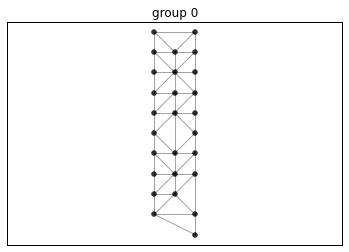
Fantastic
If we had just dropped our missing sites, we’d have huge gaping holes in our graph. Instead, we now have a bunch of edges linking past the dead sites, keeping our graph in tact.